Region connectivity and rim-to-interior depth

This tutorial introduces an expression-independent geometry module for segmented spatial data. It asks two related questions:

1. How many connected spatial structures exist inside a predefined region?

2. Where does each segment lie between the nearest boundary and the relative interior of its own connected structure?

The method uses only stable identifiers, planar physical coordinates, sample or ROI labels, and an optional region label. Marker genes and expression values do not participate in geometry construction.

1. Define radius-graph components

Let \(\mathbf{x}_i=(x_i,y_i)\) be the physical coordinate of segment \(i\). For a prespecified radius \(r\), segments \(i\) and \(j\) are adjacent when

\[\lVert \mathbf{x}_i-\mathbf{x}_j\rVert_2 \le r.\]

Connected components are the transitive closure of this adjacency relation. For example, if A–B and B–C are within \(r\), then A, B, and C belong to one component even when A–C exceeds \(r\). The implementation uses dbscan::dbscan(..., eps = r, minPts = 1), which is equivalent to connected components of the radius graph in this setting.

Components are constructed independently within each value of sample_col. Different patients, slides, or ROIs can therefore never be connected.

2. Define the buffer-union boundary

For component \(C\) and buffer fraction \(b\), stGrads constructs

\[\Omega_C(r,b) = \bigcup_{i\in C} B\!\left(\mathbf{x}_i, br\right),\]

where \(B(\mathbf{x}_i,br)\) is a circular buffer around segment \(i\). The default \(b=0.5\) makes buffers from two radius-connected points touch or overlap. The resulting polygon is consistent with the component definition.

The boundary used by the current implementation is \(\partial\Omega_C(r,b)\), including both exterior boundaries and boundaries of internal holes.

3. Define boundary depth

For segment \(i\) in component \(C\), raw boundary depth is

\[d_i = \operatorname{dist} \left( \mathbf{x}_i, \partial\Omega_C(r,b) \right).\]

Depth is normalized independently within each component:

\[\widetilde d_i = \frac{d_i-\min_{j\in C}d_j} {\max_{j\in C}d_j-\min_{j\in C}d_j}.\]

When all depths in a component are identical, stGrads assigns \(\widetilde d_i=0\). Interpretation is deliberately geometric:

• \(\widetilde d_i\approx0\): close to the nearest rim or internal-hole edge;

• \(\widetilde d_i\approx1\): relatively interior within that component.

This coordinate does not by itself represent time, differentiation, hypoxia, necrosis, or tumor evolution.

4. Load the coordinate-only demo

The package includes 2,474 segments from sample PC1_B1:

• 2,333 segments labelled PASC-S;

• 141 segments labelled PASC-A;

• no expression matrix;

• no H&E image;

• no precomputed component or depth result.

library(stGrads)
library(ggplot2)

demo_path <- system.file(
  "extdata",
  "stgrads_region_connectivity_demo.csv.gz",
  package = "stGrads"
)

region_demo <- utils::read.csv(
  gzfile(demo_path),
  stringsAsFactors = FALSE
)

dim(region_demo)
table(region_demo$region_label)

The analysis uses the pathology label only to select the region:

connectivity <- stg_region_connectivity(
  data = region_demo,
  radii = c(20, 30, 50),
  x_col = "x_um",
  y_col = "y_um",
  id_col = "CellID",
  sample_col = "sample_id",
  label_col = "region_label",
  labels = "PASC-S",
  buffer_fraction = 0.5
)

All distances are interpreted in micrometres because x_um and y_um are physical coordinates in micrometres.

5. Inspect the returned object

stg_region_connectivity() returns four linked outputs:

Output	Resolution	Main content
segments	segment × radius	component membership, raw depth, normalized depth
polygons	component × radius	sf buffer-union geometry
components	component × radius	size, centroid, area, and depth summaries
parameters	analysis	radii, input columns, filters, and geometry definitions

Key segment-level columns are:

Column	Meaning
connectivity_sample	independently processed sample or ROI
connectivity_radius	radius-graph threshold
component_id	stable component identifier within sample and radius
component_uid	sample and component combined into a global identifier
boundary_depth	distance to the nearest buffer-union boundary
boundary_depth_norm	component-specific depth scaled to \([0,1]\)

The component-count regression benchmark is:

component_counts <- aggregate(
  component_id ~ connectivity_radius,
  connectivity$components,
  function(z) length(unique(z))
)
names(component_counts)[2] <- "n_components"
component_counts

Expected output:

Radius	Components
20 µm	186
30 µm	48
50 µm	13

Component counts cannot increase as the radius increases. The sharp decrease also shows why multiscale QC is necessary: larger radii increasingly permit transitive bridging across gaps.

6. Draw the multiscale geometry panel

p_connectivity <- stg_plot_region_connectivity(
  connectivity,
  sample = "PC1_B1",
  radii = c(20, 30, 50),
  y_transform = function(y) -y,
  point_size = 0.25,
  boundary_colour = "#00CFE3",
  title = "Expression-independent PASC-S region connectivity",
  subtitle = paste(
    "Cyan lines: buffer-union boundaries;",
    "colour: component-normalized boundary depth"
  )
)

p_connectivity

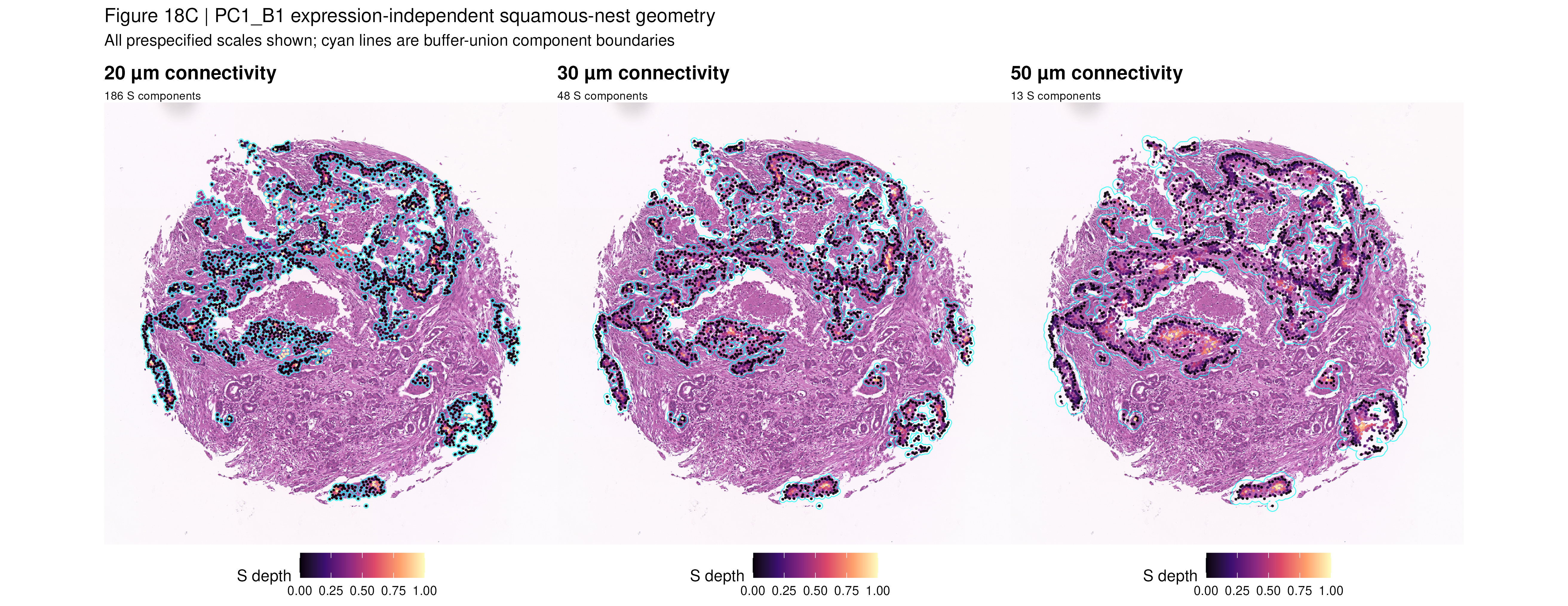
Result: the 20 µm graph fragments the annotated region into many small components, 30 µm gives an intermediate representation, and 50 µm permits substantial chain-like bridging. Cyan lines are buffer-union boundaries; purple-to-yellow point colour represents increasing normalized depth.

The displayed Figure 18C uses an H&E background available in the application analysis. The package demo intentionally contains only coordinates and labels.