Visium HD Morphometry and Mixed-Unit Refinement

This tutorial presents the pathology-aware workflow introduced in stGrads 2.0. It follows the same goal → key arguments → runnable code → figure → interpretation structure used by the original stGrads tutorials.

The analysis connects six evidence layers:

segmented Visium HD cells → cell and nuclear morphometry → RCTD mixed-unit annotation → local spatial support → dual marker programs → composite-segment prioritization.

The terminology is deliberate. An RCTD mixed unit contains evidence for two cell types, whereas a spatially supported mixed unit additionally has nearby singlets matching both constituent types. Neither term alone proves direct membrane contact.

---

1. Install and load stGrads 2.0

Goal: load the package and the plotting dependencies used in this tutorial.

remotes::install_github("yifanfu01/stGrads")

library(stGrads)
library(ggplot2)
library(patchwork)
library(Matrix)

For a local source checkout:

remotes::install_local("/PATH/TO/stGrads2")

---

2. Load the publication-ready demo

Goal: load a compact, real segmented Visium HD region that can regenerate the tutorial figures without shipping a whole-slide object.

data("stgrads_hd_pc1_a2_roi_demo")
demo <- stgrads_hd_pc1_a2_roi_demo

dim(demo$counts)
# 18085 genes x 678 segmented cells

dim(demo$polygons)
# 10864 polygon vertices x 4 columns

table(demo$metadata$duct2_fib_status)

The demo contains only the selected region selected, for the whole slide data, please refer the original manuscript :

• complete sparse counts from the Spatial.Polygons assay;

• 678 cell centroids and segmentation polygons;

• a cropped H&E image;

• RCTD singlet and mixed-unit labels;

• cell and nuclear morphology;

• pre-crop spatial-support results for mixed units.

*The compressed package object is approximately 0.57 MB.

metadata <- demo$metadata
polygons <- demo$polygons

image_path <- stg_demo_image_path(demo)

p_he <- stg_plot_hd_he(demo) +
  geom_polygon(
    data = polygons,
    aes(x, y, group = CellID),
    fill = NA,
    color = "white",
    linewidth = 0.12
  )

p_he

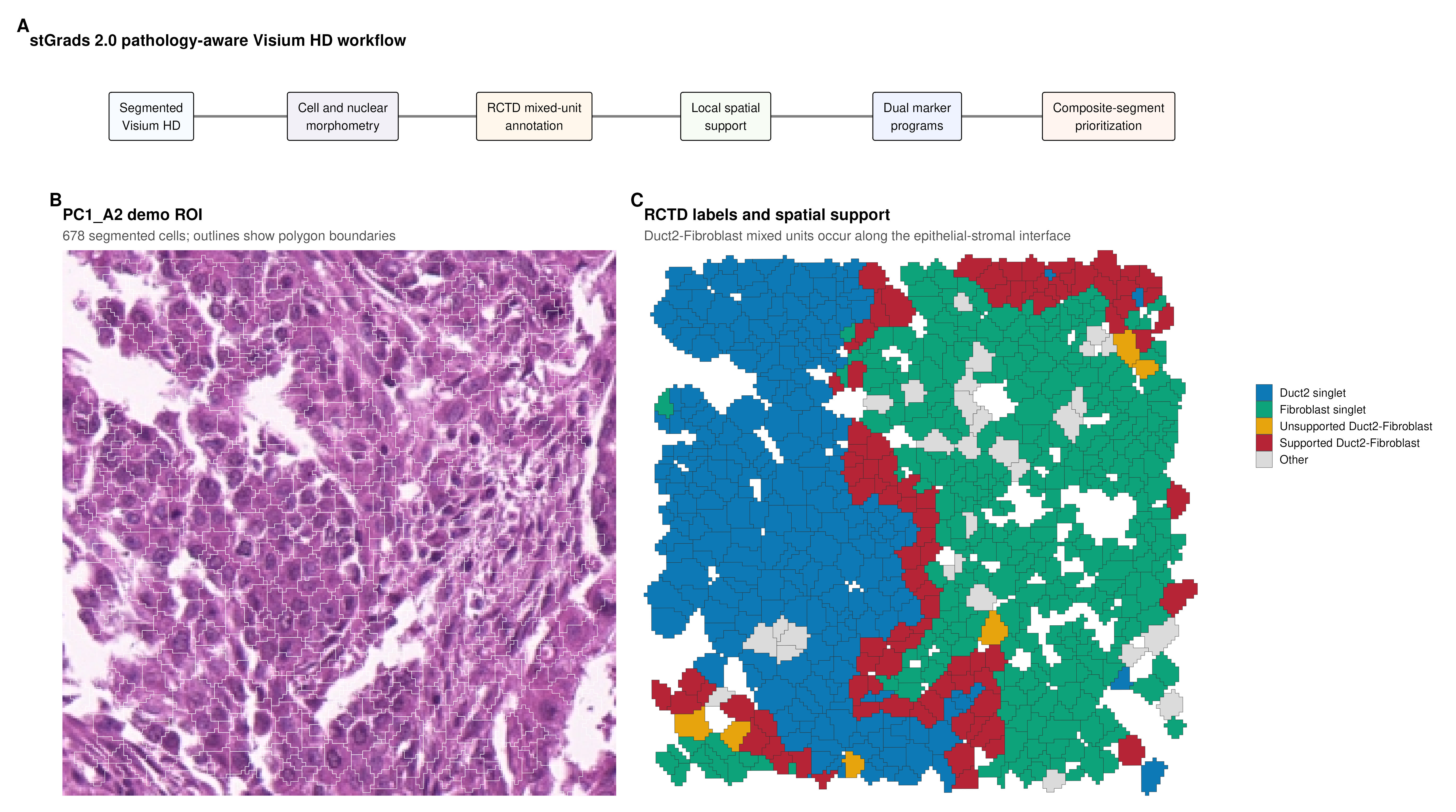
Result: the ROI contains a Duct2-rich epithelial region adjacent to a fibroblast-rich stromal region. Duct2–Fibroblast mixed units concentrate near their interface, making this crop useful for demonstrating spatial support and segmentation refinement.

---

3. Keep image coordinates and analytical coordinates separate

The demo intentionally stores two coordinate systems.

Purpose	Columns	Unit
Polygon and H&E plotting	x, y in demo$metadata and demo$polygons	full-resolution pixels
Distance-based analysis	centroid_x_um_cell, centroid_y_um_cell	micrometres

Use full-resolution pixels to align polygons with H&E. Use micrometre coordinates for support radii, nearest-neighbour distances, and spatial gradients. Mixing these systems silently changes the biological radius.

For a previously saved Seurat object, the compatibility layer adds standardized coordinates without removing assays, images, reductions, or metadata:

object <- readRDS("previous_spatial_object.rds")
object <- stg_upgrade_object(object)

---

4. Standardize undirected RCTD pairs

Goal: convert first_type and second_type into one stable, undirected pair label.

metadata <- stg_annotate_rctd(metadata)

stg_canonical_pair(
  c("Duct2", "Fibroblast"),
  c("Fibroblast", "Duct2")
)
# Both entries are "Duct2__Fibroblast".

Mathematically, the pair is a set rather than an ordered tuple:

\[\{i,j\}=\{j,i\}.\]

This convention prevents the same biological pair from appearing twice in summaries or triangular heatmaps.

---

5. Evaluate local spatial support

Goal: require both constituent cell types of an RCTD mixed unit to be represented by nearby singlets.

For mixed unit \(u\) with constituent types \(a_u\) and \(b_u\), define

\[d_a(u)=\min_{s:\,T_s=a_u}\lVert \mathbf{x}_u-\mathbf{x}_s\rVert_2, \qquad d_b(u)=\min_{s:\,T_s=b_u}\lVert \mathbf{x}_u-\mathbf{x}_s\rVert_2.\]

With radius \(r_0=30\,\mu\mathrm{m}\), the support indicator is

\[I_{\mathrm{support}}(u) =\mathbb{1}\{d_a(u)\le r_0\} \mathbb{1}\{d_b(u)\le r_0\}.\]

For an uncropped sample, calculate support as follows:

support <- stg_doublet_spatial_support(
  metadata = metadata,
  coordinates = metadata,
  radius = 30,
  sample_col = "MatchKey",
  cell_id_col = "CellID",
  x_col = "centroid_x_um_cell",
  y_col = "centroid_y_um_cell",
  coordinate_cell_col = "CellID"
)

The package demo provides demo$spatial_support, calculated before the ROI was cropped. This preserves valid neighbours immediately outside the displayed region and avoids crop-edge bias:

support <- demo$spatial_support

metadata <- stg_add_spatial_support(
  metadata,
  support,
  cell_id_col = "CellID"
)

target_support <- subset(
  support,
  doublet_pair == "Duct2__Fibroblast"
)

table(target_support$both_types_supported)
# FALSE  TRUE
#     6    90

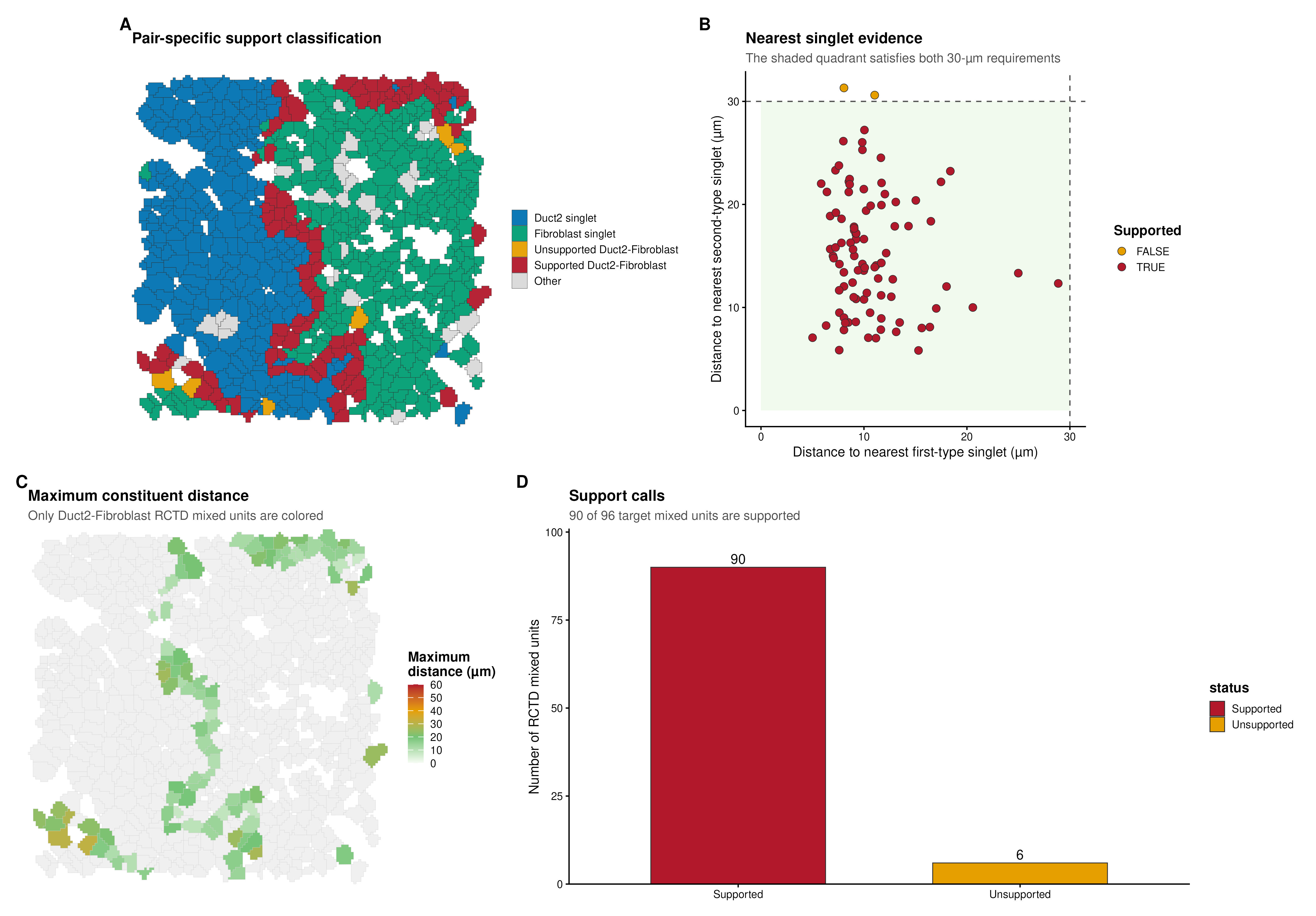
Result: 90 of 96 Duct2–Fibroblast mixed units have both constituent singlet types within 30 µm in the pre-crop spatial context. This supports local compatibility; it does not establish membrane contact.

---

6. Replace single markers with deterministic marker programs

Goal: identify units containing concordant epithelial and fibroblast transcriptional signals while reducing sensitivity to single-gene dropout.

First normalize the complete polygon count matrix:

log_expression <- stg_normalize_counts(
  demo$counts,
  scale_factor = 1e4
)

For marker set \(G_m\), stGrads standardizes each gene across cells and averages the available markers:

\[P_m(u)=\frac{1}{|G_m|}\sum_{g\in G_m} \frac{X_{gu}-\bar X_g}{s_g}.\]

The implementation is deterministic and does not randomly sample control genes:

programs <- stg_marker_programs(
  log_expression,
  gene_sets = list(
    Duct2 = demo$duct2_markers,
    Fibroblast = demo$fibroblast_markers
  )
)

metadata$Duct2_program <- programs[metadata$CellID, "Duct2"]
metadata$Fibroblast_program <- programs[metadata$CellID, "Fibroblast"]

Each program is independently rescaled to \([0,1]\). The default joint signal uses the fuzzy-set intersection:

\[J(u)=\min\{\widetilde P_{\mathrm{Duct2}}(u), \widetilde P_{\mathrm{Fibroblast}}(u)\}.\]

Therefore, one high program cannot compensate for an absent second program.

metadata$program_overlap <- stg_program_overlap(
  metadata$Duct2_program,
  metadata$Fibroblast_program,
  method = "minimum"
)

stg_plot_polygon_feature(
  metadata,
  polygons,
  feature = "program_overlap",
  colors = c("#FFF7EC", "#FDD49E", "#FC8D59", "#D7301F", "#7F0000"),
  limits = c(0, 1)
)

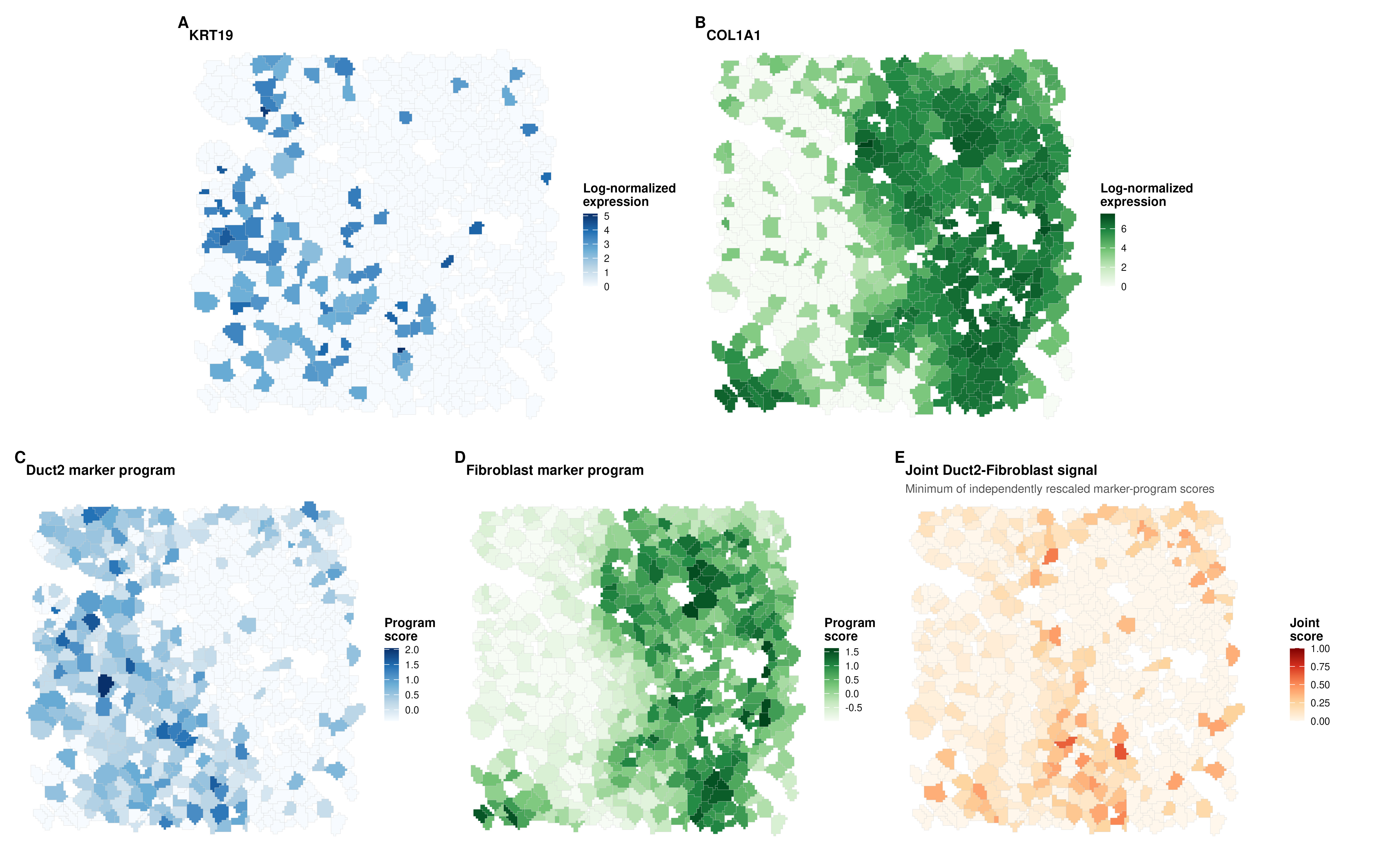
Result: KRT19 and COL1A1 provide an intuitive single-gene view, whereas the program scores provide the more stable evidence layer used for refinement. The joint score highlights a subset of cells near the epithelial–stromal interface.

---

7. Combine cell and nuclear morphology

Goal: distinguish cell enlargement from nuclear enlargement and avoid interpreting cell area alone as evidence of a composite segment.

The most useful paired quantities are

\[A_{\mathrm{cell}},\qquad A_{\mathrm{nuc}},\qquad f_{\mathrm{nuc}}=\frac{A_{\mathrm{nuc}}}{A_{\mathrm{cell}}}, \qquad R_{N:C}=\frac{A_{\mathrm{nuc}}} {A_{\mathrm{cell}}-A_{\mathrm{nuc}}}.\]

morphology_fields <- metadata[, c(
  "CellID",
  "area_um2_cell",
  "area_um2_nuc",
  "nucleus_fraction",
  "nc_ratio",
  "circularity_cell",
  "boundary_complexity_cell",
  "nucleus_centroid_displacement_norm"
)]

summary(morphology_fields[, -1])

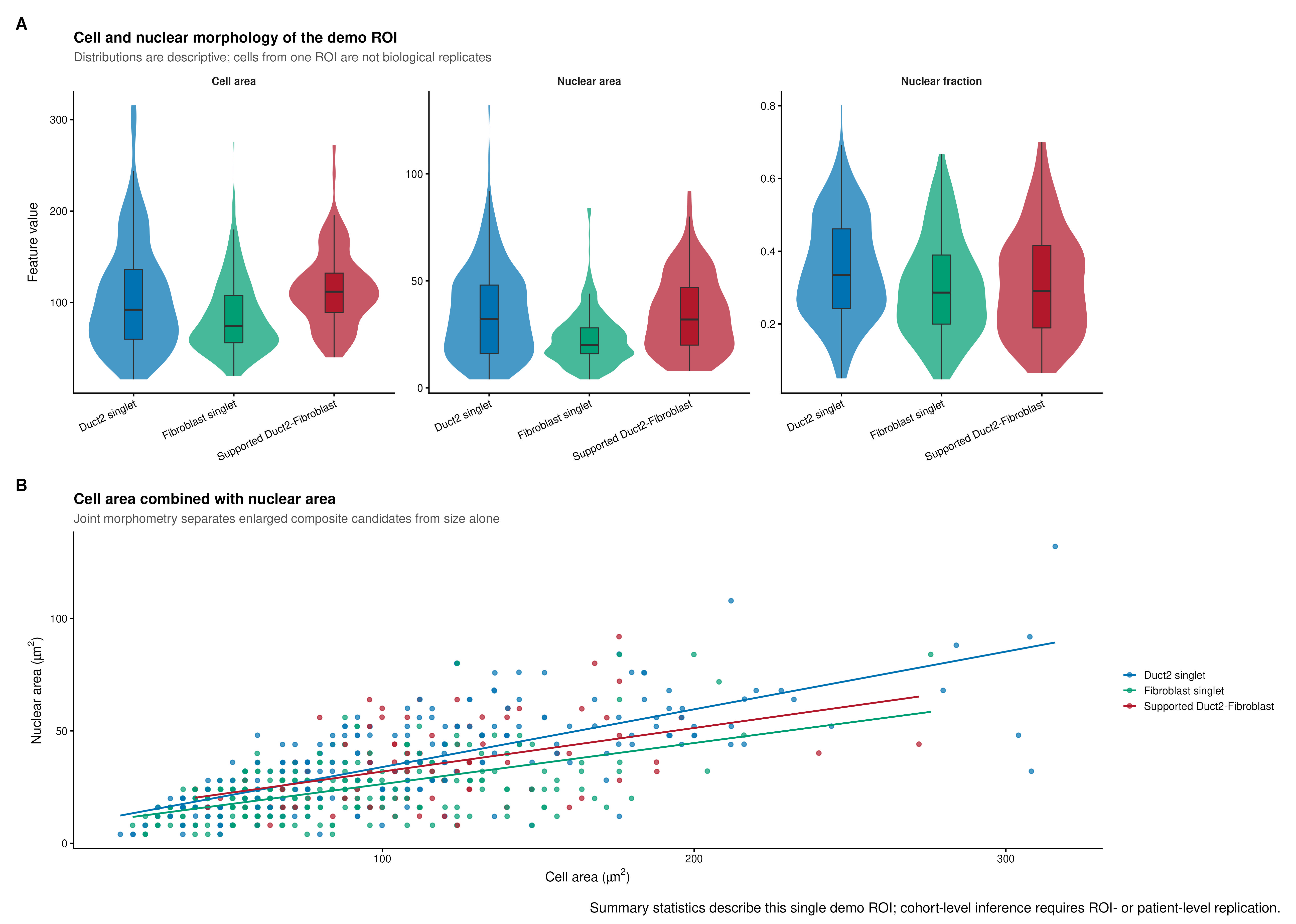
Result: supported Duct2–Fibroblast mixed units show a shifted distribution of cell and nuclear measurements relative to the two singlet populations. The two-dimensional cell-area/nuclear-area view is more informative than a single size feature.

These distributions are descriptive. Cells within one ROI are not independent biological replicates, so the tutorial reports counts, medians, and interquartile ranges rather than cell-level inferential P values. Cohort-level testing should use ROI or patient as the replication unit.

---

8. Integrate evidence for composite-segment prioritization

Goal: rank RCTD mixed units for image review or nucleus-aware re-segmentation.

refined <- stg_refine_doublets(
  metadata,
  support_col = "both_types_supported",
  overlap_col = "program_overlap",
  sample_col = "MatchKey"
)

table(refined$stg_refinement_class, useNA = "ifany")

Each continuous evidence component is robustly standardized within sample and mapped to \([0,1]\). For unit \(u\), the integrated score is

\[C(u)= \frac{\sum_{k\in\mathcal A_u}w_k e_k(u)} {\sum_{k\in\mathcal A_u}w_k},\]

where \(\mathcal{A}_u\) is the set of available evidence components. The default weights are:

Evidence	Weight
spatial support	2.0
cell area	1.0
nuclear area	0.5
transcript count	1.0
detected genes	1.0
dual marker-program overlap	2.0

Default classes are low evidence \(C<0.45\), moderate evidence \(0.45\le C<0.70\), and high confidence \(C\ge0.70\).

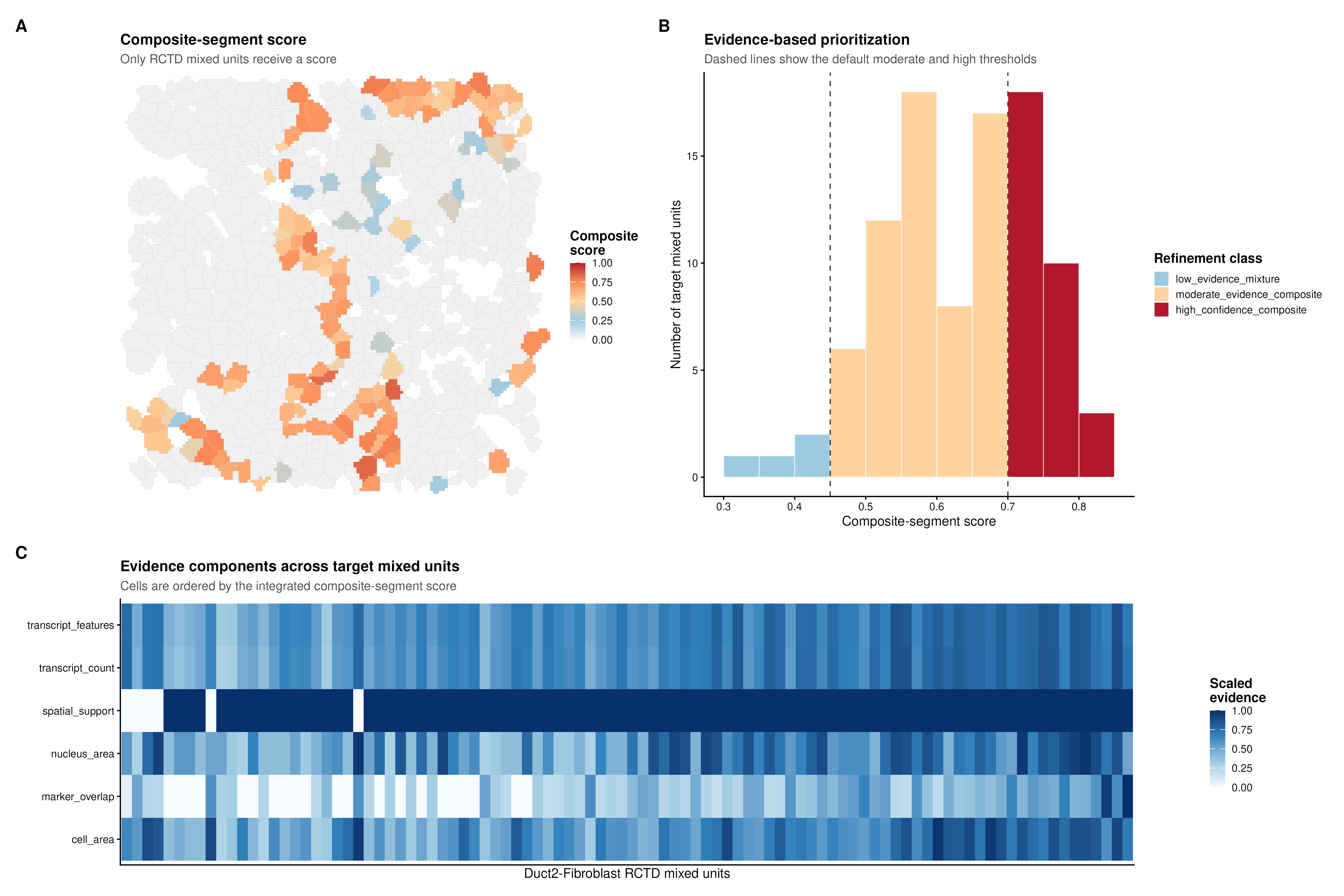
Result: spatial support and dual marker evidence move many interface mixed units into the moderate- or high-confidence categories. The function ranks candidates but does not alter polygon geometry automatically.

---

9. Extend the original stGrads gradient framework to morphology

Goal: test whether fibroblast morphology or transcriptional programs vary with distance from Duct2 singlets.

gradient <- stg_spatial_gradient(
  object = metadata,
  label_col = "first_type",
  reference = "Duct2",
  query = "Fibroblast",
  sample_col = "MatchKey",
  x_col = "centroid_x_um_cell",
  y_col = "centroid_y_um_cell",
  cell_id_col = "CellID",
  max_distance = 150,
  decay = "exponential"
)

head(gradient)

For query cell \(u\), the nearest-reference distance is

\[d(u)=\min_{r\in\mathcal R}\lVert\mathbf{x}_u-\mathbf{x}_r\rVert_2,\]

and the exponential cumulative strength within radius \(d_{\max}\) is

\[S(u)=\sum_{r\in\mathcal R} \exp[-d(u,r)]\,\mathbb{1}\{d(u,r)\le d_{\max}\}.\]

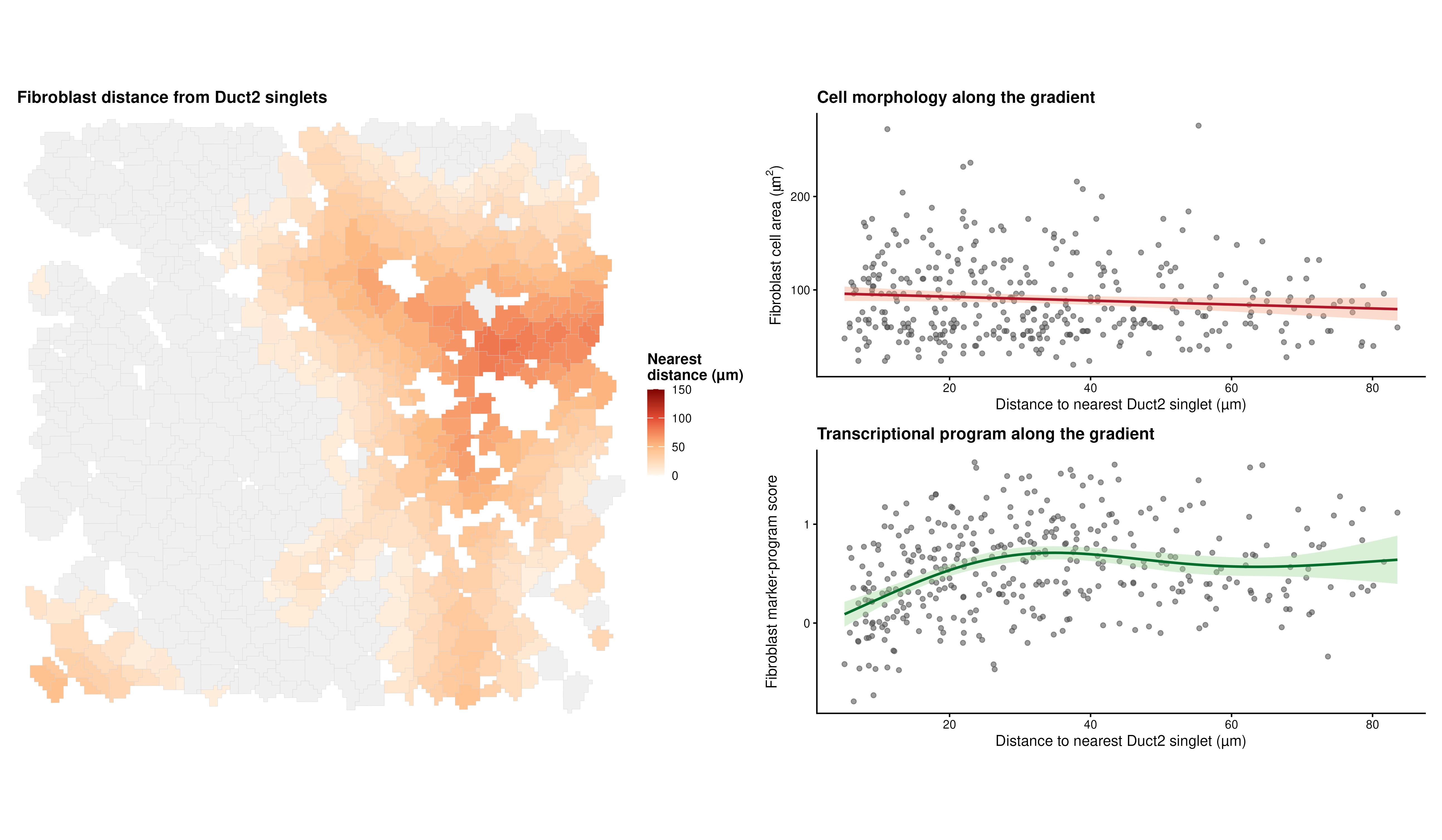
Result: the demo illustrates how previous stGrads v1.0 function used in new version package, that is, spatial distance, cell morphology, and a fibroblast transcriptional program can be displayed in one coherent analysis.

---

10. Calculate undirected observed-to-expected pair enrichment

Goal: compare the observed number of each mixed-unit pair with the number expected from local singlet composition.

##DO NOT RUN

enrichment <- stg_pair_enrichment(
  metadata,
  sample_col = "MatchKey",
  condition_col = "Condition",
  min_singlet_cells = 100,
  min_expected = 5,
  min_expected_fraction = 1e-4
)

enrichment$condition[, c(
  "doublet_pair",
  "observed",
  "expected",
  "oe_raw",
  "log2_oe",
  "estimable"
)]

For ROI \(r\), let \(S_{ir}\) be the type-(i) singlet count and \(p_{ir}=S_{ir}/\sum_k S_{kr}\). For an undirected heterotypic pair \(i<j\),

\[q_{ijr} =P(\{i,j\}\mid X\ne Y) =\frac{2p_{ir}p_{jr}}{1-\sum_kp_{kr}^2}, \qquad E_{ijr}=D_rq_{ijr}.\]

The denominator uses all singlet types before pair-specific filtering. Across eligible ROIs, observed and expected counts are summed before taking their ratio:

\[R_{O/E,ijc}=\frac{\sum_r O_{ijr}}{\sum_r E_{ijr}}, \qquad L_{ijc}=\log_2R_{O/E,ijc}.\]

No pseudocount is added to the primary effect size. An estimate is displayed only when

\[E_{ijc}\ge\max\left(5,10^{-4}N_{ijc}\right).\]

stg_plot_pair_triangle(
  enrichment$condition,
  value_col = "log2_oe",
  show_counts = TRUE
)

Result: Cause the demo ROI only contains Duct2–Fibroblast mixed units, this value only exhibite output data format.

The complete derivation and output-column definitions are provided in (Advanced)Mathematical definition.

---

11. Reproducibility files

packageVersion("stGrads")
sessionInfo()